Kordil Geodesy Tools
Advanced User Manual
A practical technical reference for coordinate transformations, parameter estimation, least-squares adjustment, uncertainty and error investigation.
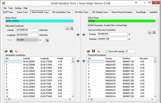 1234
- 1 Operation tab.
- 2 Source datum and input.
- 3 Target datum/projection.
- 4 Batch transformation and direction controls.
Contents
Distinguish software functionality from theoretical methods
Kordil Geodesy Tools — KGTis a Windows desktop application combining coordinate transformation and survey-data preparation in one workspace. Developed by Kordil, it covers single-point and file-based transformations, parameter estimation from common points, image georeferencing and selected hydrographic processing tasks.
This manual explains more than button locations. It describes the selected model, the assumptions under which a solution is valid and how to test the result. Classical geodetic formulas are provided for technical training; source code and proprietary software architecture are not published.
| Module / operation | Verified scope | Do not assume |
|---|---|---|
| ECEF Trans | Latitude, longitude, ellipsoidal height ↔ geocentric XYZ | Automatic recognition of orthometric height |
| Datum Trans / 3-D Coordinates Trans | Transformation using defined ellipsoids and seven parameters | Automatic selection of official grids/epoch transformations for every datum pair |
| TM/UTM/GK Trans | Customisable Transverse Mercator parameters | Reliable identification of zone and hemisphere from coordinates alone |
| 2-D Similarity / Affine | Four/six parameters respectively from common points; forward and inverse application | Joint adjustment of source and target covariances |
| Datum Param Estimation | Seven-parameter estimation and reporting from common 3D points | Verified convergence for unrestricted rotations or automatic gross-error removal |
| KMZ DXF Tools / image georeferencing | Table, map and CAD exchange; BMP georeferencing | Lossless preservation of every CAD object and raster model |
| SonarMagic | Matching timestamped positions and soundings; depth processing | Full multibeam ray tracing, motion compensation or automatic hydrographic acceptance |
Set up a reproducible job
- Define the job: source/target CRS, horizontal and vertical datums, epoch, units, axis order and acceptance criteria.
- Protect the input: leave the master file unchanged and separate working and output folders.
- Select the operation tab: format/projection conversion within a datum, transformation between datums, or parameter estimation?
- Verify datum and projection: load A/B definitions from files or enter them from an authoritative source. A retained setting is not necessarily correct merely because it came from a previous session.
- Run a small test: use a known point and a short sample file to check columns, direction and numeric format.
- When estimating parameters: load common points, enable reporting, solve the model and complete residual and independent-check analysis.
- Batch application: transform the production file with verified parameters. Do not confuse estimation points with points to be transformed.
- Export and acceptance: verify row counts, IDs, extent, units and check differences; archive definition files and the report together.
Interface logic
Upper tabs select the operation family; coloured datum panels show the definitions in use. Single-point fields are for quick checks and lower tables for batch transformations. Check arrow direction against the actual source-to-target direction. Names and colours may differ in older help images. Use menus and tooltips rather than identifying an icon solely from an old screenshot.
In parameter-estimation tabs, enable Report or the calculation-details option before solving. Save the report separately. Use your own job record to confirm that displayed parameters belong to the latest successful computation.
Coordinate system, datum, CRS and epoch
A coordinate system defines axes, units and geometric rules. A datum relates that system to the physical Earth. A coordinate reference system (CRS) defines these together. Two files both labelled “X, Y” need not use the same reference system.
Conversion / coordinate conversion
Representation changes without changing datum: ellipsoidal ↔ ECEF or geographic ↔ projected coordinates. Although the operation is mathematical, input and definition uncertainties do not disappear.
Transformation / reference-frame transformation
Empirical parameters relate different datums or frames. Their source data, area of validity, direction and uncertainty matter.
Why does epoch matter?
Coordinates in dynamic frames depend on time. Coordinates for different epochs, earthquakes or deformation effects may not be reconciled by seven constant parameters alone. The same ellipsoid name does not make two datums equivalent. Do not assume that the reviewed KGT workflow automatically applies velocity fields, a time-dependent 14-parameter model or deformation grids.
Distinguishing heights
h = H + N · h: ellipsoidal height · H: orthometric height · N: undulation of the appropriate geoid model
This relation explains the physical concept; it does not mean KGT automatically selects the correct geoid file. Normal heights require a consistent definition using the relevant height anomaly and quasigeoid model. Do not enter a local water-level datum as ellipsoidal height.
Georeferencing a raster is not a vertical-reference transformation. “Geo” in a menu, file or module name does not prove a national geoid calculation is being performed.
A file being readable does not mean it was interpreted correctly
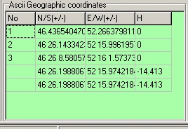
| Check | Application |
|---|---|
| Axis order | Latitude/longitude in geographic tables; E/N in projections; X/Y/Z in 3D tables. Record labels with their physical meaning. |
| Angle format | DD: 40.5; DM: 40 30; DMS: 40 30 0. Decimal minutes and decimal degrees are not the same. |
| Sign | Use the appropriate negative sign for south/west. Test specifically for loss of sign on coordinates between zero and minus one degree. |
| Decimal notation and delimiter | Clearly define decimal points/commas and column delimiters in the file. Resolve decimal-comma ambiguity in CSV. |
| IDs and duplicates | Match common points by physical identity. A duplicated ID or row is not an independent observation. |
| Missing height | Zero, blank, unknown and a genuine zero have different meanings. Never replace missing heights with zero in 3D estimation. |
| Precision | The number of output decimals is not accuracy. Rounding intermediate results and reusing them accumulates errors. |
Test with a small file
ID LAT LON h
P01 40.500000000 29.250000000 50.000
P02 40.501000000 29.251000000 51.000
This fictional example illustrates column meanings. Test header and delimiter support with the selected reader. File readers may support different formats. Use the preview to check that headers, comments or numeric point IDs are not misread as coordinate columns. Older supplied test files may intentionally contain faulty or annotated records; they are not approved field data.
Angle conversion
DD = sign × (|D| + M/60 + S/3600)
1″ = π / 648000 rad
1 gon = 0.9°
NMEA ddmm.mmmm → D + minutes/60
Apply one sign to the entire DMS angle. Do not interpret −0° 30′ using only the integer degree value. Minutes and seconds must satisfy 0 ≤ value < 60. 40.3000° and 40°30′ are different positions.
ECEF model and inverse-solution checks
ECEF is an Earth-centred, Earth-fixed Cartesian system. X points towards the intersection of the equator and prime meridian, Y towards 90° east on the equator, and Z towards the North Pole. Latitude φ, longitude λ and ellipsoidal height h must refer to the same ellipsoid.
f = 1 / (1/f)                 e² = f(2 − f)
ν(φ) = a / √(1 − e² sin²φ)
X = (ν + h) cosφ cosλ
Y = (ν + h) cosφ sinλ
Z = [ν(1 − e²) + h] sinφ
a is the semi-major axis and f is flattening. The interface's Inverse flattening is 1/f; do not enter f directly. Formulas use radians, while user input follows the selected degree format.
 12
- 1 Latitude, longitude and ellipsoidal height.
- 2 XYZ on the same ellipsoid.
Inverse conversion
A general inverse solution uses p = √(X²+Y²) and λ = atan2(Y,X); latitude and height follow an appropriate closed-form or iterative method. The reviewed KGT inverse path is iterative. Each algorithm's behaviour at poles, the origin and quadrant boundaries must be tested separately. Availability of an inverse conversion is not an unconditional guarantee for every numerical extreme.
Minimum validation set
- At the equator and zero longitude, h=0 gives X≈a, Y≈0, Z≈0.
- Longitude quadrants for north/south and east/west combinations.
- Forward–inverse closure at typical points in the working area.
- Controlled error behaviour near the poles and for invalid input near the Earth's centre.
- Comparison of the same point with an independent calculation using matching definitions.
Using the same incorrect definition in both directions may yield a small closure error. An independent known-point test is essential.
Datum definition, transformation direction and rotation convention
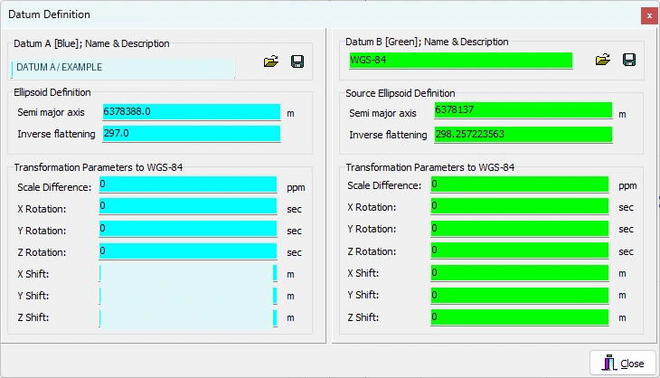 123
- 1 a and 1/f: ellipsoid geometry.
- 2 Datum A transformation parameters to WGS 84.
- 3 Datum B transformation parameters to WGS 84.
Some project-specific values are hidden. Do not copy visible values to another project; follow field labels and operation direction.
Development screen archive, 10 February 2026; prepared for training.Standard seven-parameter model
rT = t + m R rS
m = 1 + dS × 10⁻⁶
rS, rT: source and target XYZ vectors
t: (tX, tY, tZ) translations [m]
dS: scale difference [ppm]
R: rotation matrix; angle units and convention are defined
One ppm is one part per million, corresponding to about 1 mm of scale effect over 1000 m. Confusing degrees, arcseconds and radians produces very large errors. KGT's datum screen shows rotations in arcseconds, translations in metres and scale difference in ppm.
Transformation chain through WGS 84
The logical geographic datum chain is: source-ellipsoid φλh → source XYZ → source datum to WGS 84 → WGS 84 to target datum → target-ellipsoid φλh. Parameters defined from the target datum to WGS 84 are applied inversely when entering the target datum. Simply subtracting A and B parameters does not generally yield the correct composed transformation.
Coordinate Frame and Position Vector
These common conventions interpret identical rotation values with opposite signs. One small-angle Coordinate Frame form is:
R_CF ≈ [  1    +rz   −ry ]
       [ −rz    1    +rx ]
       [ +ry   −rx    1  ]
R_PV ≈ R_CFᵀ  (compare rotation signs for the same physical relationship)
KGT's classical help specifies the Coordinate Frame approach; the numerical calculation also contains full trigonometric rotations. Do not match a parameter set from another program by the name “Helmert” alone. Record source/target direction, angle sequence, rotation convention, linearised/full model and scale definition together. For large angles, changing signs alone does not make different Euler rotation sequences equivalent.
Inverse operation
rS = (1/m) Rᵀ (rT − t) [if R is orthogonal and m ≠ 0]
Merely reversing the signs of seven parameters, without subtracting translations from the target vector, is not the general inverse transformation. Use KGT's direction controls with an independent control point. Definition files may be saved as .datum files; archive operation metadata separately.
Transverse Mercator, UTM and Gauss–Krüger
TM is a projection family; UTM and Gauss–Krüger are implementations with specific zones, scales and coordinate arrangements. “Convert to UTM” is insufficient without defining central meridian λ₀, latitude of origin φ₀, scale k₀, false easting FE and false northing FN.
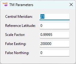
A = (λ − λ₀) cosφ       T = tan²φ       C = e′² cos²φ
E ≈ FE + k₀ ν [A + (1 − T + C)A³/6 + …]
N ≈ FN + k₀ [M(φ) − M(φ₀)
             + ν tanφ (A²/2 + (5 − T + 9C + 4C²)A⁴/24 + …)]
M is the meridian arc and e′ the second eccentricity. This series illustrates the model structure; do not use the truncated expression as a production calculation. KGT's TM path uses a series expansion. Independently test validity and stability far from the central meridian, near the poles and for unusual projections.
Distinguish standard UTM from custom local TM
Common UTM uses 6° zones, k₀=0.9996 and FE=500000 m, with false northing for the southern hemisphere defined separately. In ordinary regions, the zone formula is λ₀=6z−183°. Special zone arrangements exist, so do not identify a CRS from this formula alone. Gauss–Krüger zone width, prefix and scale may vary by national practice.
Grid versus ground
Dgrid ≈ k × [R/(R+h)] × Dground
combined factor ≈ projection scale × elevation factor
This approximate relation helps interpret short horizontal distances; do not compare slope distance directly with grid length. Meridian convergence is the directional difference between true and grid north. Projected coordinates from KGT do not imply that local point scales, convergence or ground-to-grid reductions are also reported. Include these effects in the engineering-network error budget.
2D similarity: change the coordinate frame while preserving shape
Similarity transformation contains two translations, one rotation and one scale shared by both axes. It preserves angles and length ratios. It is a first candidate for adapting local engineering coordinates to another planar system when shape must be retained. One similarity transformation cannot remove all spatially varying distortion between different projections over a large area.
XT = tx + a XS + b YS
YT = ty − b XS + a YS
a = s cosθ        b = s sinθ
s = √(a²+b²)      θ = atan2(b,a)
q = [tx, ty, a, b]ᵀ
Signs follow KGT's 2D model direction here. Do not infer angle signs by assuming conventional X-east/Y-north axes or downward-increasing image Y. Test the physical effect of positive θ against a known direction.
Solution and application
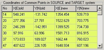
- Open 2-D Similarity Trans and use a common-point file or table input.
- At least two distinct points are required. The minimum alone provides no residual-based model validation. Use additional common points surrounding the work area.
- Enable reporting and calculate parameters. Do not mistake retained values for a new solution.
- Recalculate each control point using the parameters and subtract its target coordinates. Confirm the report columns give the same differences.
- Validate with points excluded from the solution before applying forward or inverse transformation to the production file.
Inverse model and limiting cases
u = XT − tx          v = YT − ty
XS = (a u − b v)/(a²+b²)
YS = (b u + a v)/(a²+b²)
A scale near zero makes the transformation meaningless. Test angle quadrants, zero rotation with non-unit scale, rotations near ±90° and inverse calculations specifically. A mathematical model may define these cases, but do not assume parameter display and every inverse code path behave equivalently at all extremes.
2D affine: independent scales and skew
XT = a0 + a1 XS + a2 YS
YT = b0 + b1 XS + b2 YS
q = [a0, a1, a2, b0, b1, b2]ᵀ
B = [a1 a2; b1 b2]           det B = a1 b2 − a2 b1
Affine transformation preserves parallelism but generally not angles or length ratios. It can include independent axis scales, rotation, skew and, where applicable, reflection. Uses include old sheets/rasters, planar local systems with unequal scales and geometrically distorted engineering drawings. It is not a physical model that universally represents a geodetic datum difference.
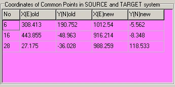
Model selection
Establish the geometric justification first. Affine transformation may be appropriate if systematic similarity residuals can be explained by unequal axis scales. Do not add parameters merely because residuals shrink: extra parameters can absorb mismatched control points or local defects. With identical data and equal weights, affine internal fit will look at least as good as similarity; this does not establish better external accuracy.
Application checks
- At least three non-collinear common points; in practice, use redundant points surrounding and checking the centre of the area.
- Redundancy f=2n−6. With three points f=0, so variance factors and residual-based tests cannot be obtained.
- If det B is near zero, inversion is unstable. A negative determinant may indicate reflection; investigate axis order or point matching if this is unexpected.
- Do not assume 2D transformations adjust heights. In the reviewed affine/similarity application paths, the height column is carried through unchanged.
A1, A2, B1 and B2 are generally dimensionless; A0/B0 use coordinate units. Axis scales can be derived from transformed source basis-vector lengths: sX=√(a1²+b1²), sY=√(a2²+b2²). For orthogonal source axes, the dot product of target basis vectors describes skew. Since several rotation/shear decompositions are possible, state the decomposition convention used in the report.
Datum parameters from common 3D points
Datum Param Estimationestimates translations, rotations and scale from two known XYZ sets. “Inverse Helmert” here means determining unknown parameters from coordinates, not merely transforming points backwards using known parameters.
- Confirm common points represent the same physical location, compatible epochs and the same units in both systems.
- Prepare seven columns: ID, first-system X/Y/Z and other-system X/Y/Z. Confirm source/target interpretation against the selected screen and report; the label Xt alone is insufficient.
- Load at least three geometrically independent common points. Three nearly collinear points do not provide suitable 3D determinability.
- Enable the report and estimate parameters. Test the direction they represent using two known points.
- Check units and direction when transferring translations, ppm and arcseconds to the target datum definition.
- Perform at least one independent check and a forward–inverse closure test. Do not generalise a solution with inadequate spatial or height distribution.
Distinguish linearisation from full rotation
The general model rT=t+sRrS is nonlinear. The classical small-angle approximation linearises rotations. More general estimation forms a Jacobian A=∂F/∂q around approximate values q₀ and updates the solution with corrections. Using a full trigonometric R alone does not demonstrate a well-converged nonlinear adjustment.
Common-point quality
ECEF points over a small site cluster around nearly the same large geocentric vector. Parameters may be strongly correlated; very small internal residuals do not establish seven physically reliable parameters. Do not derive a national datum change from a few narrowly distributed points and apply it nationally. Consider authoritative transformation grids, regional models and epoch corrections first.
Least-squares adjustment: what is minimised?
Least-squares adjustment minimises the weighted sum of squared residuals under the selected functional and stochastic models. It does not automatically turn a wrong model, datum or gross error into a correct result. “Adjusted” alone is not sufficient evidence that a solution is reliable.
Linear model and sign convention
l + v = A q
q̂ = arg min (Aq − l)ᵀ P (Aq − l)
N = Aᵀ P A                  n = Aᵀ P l
N q̂ = n                     v̂ = A q̂ − l
Aᵀ P v̂ = 0
In this manual, v means computed minus observed . Other sources may use the opposite sign. The sum of squares is unchanged, but residual-map directions reverse. A is the design matrix, q the unknown parameters, l the observation vector and P the weight matrix. With full column rank, q̂=(AᵀPA)⁻¹AᵀPl holds theoretically. Numerical practice may favour QR or SVD over explicit inversion; this does not claim that KGT uses those methods.
Two observation rows for similarity
[XT]   [1 0  XS  YS] [tx]
[YT] = [0 1  YS −XS] [ty] + observation error
                       [a]
                       [b]
“Observation error” here belongs to l−Aq; the correction v defined above has the opposite sign. Each point contributes two scalar equations. Affine rows are [1 XS YS 0 0 0] and [0 0 0 1 XS YS]. In 3D, each point provides three equations and derivatives of the rotation model form A.
Degrees of freedom and posterior variance
f = m − rank(A)       [at full rank f = m − p]
SSE = v̂ᵀ P v̂
s₀² = SSE / f         [f > 0]
s₀ = √(SSE/f)
| Model | Scalar equations m | Parameters p | f at full rank |
|---|---|---|---|
| 2D similarity | 2n | 4 | 2n−4 |
| 2D affine | 2n | 6 | 2n−6 |
| 3D Helmert | 3n | 7 | 3n−7 |
n is the number of points and m the number of scalar observations. At f=0 an exact solution may exist, but s₀ cannot be estimated from the data. With rank deficiency, m−p alone is insufficient; investigate datum defects or geometry. Repeating the same point in a file does not physically increase independent information.
Moving to a nonlinear model
l = F(q) + ε
w = l − F(q₀)          A = ∂F/∂q |q₀
A δq ≈ w               q_new = q₀ + δq
A general iterative method monitors correction norms, the objective function, physical parameter changes and rank. With different units, one numeric threshold for every parameter may be inappropriate. This is theoretical and does not imply KGT has a convergence manager in its interface.
Weights: trust good observations, for the right reasons
The functional model defines expected coordinate relationships; the stochastic model defines observation uncertainty and correlation. The same geometry with different weights may produce different parameters. Weight a point according to independent measurement-quality information, not because you dislike its result.
Cov(l) = σ₀² Qll
P = Qll⁻¹
for independent observations: Pii = σ₀² / σi²
σ₀² is a common reference variance. Where full covariance is known, select a consistent scale. P=I assumes equal relative confidence in every scalar component and zero correlation. Equal weighting does not prove equal accuracy of every field point.
The reviewed similarity, affine and 3D estimation paths use P=I. Adding a “sigma” column does not automatically create a weighted solution. Automatic use of full point covariances, inter-axis correlations or source-coordinate errors has not been verified in these paths.
When both systems contain errors
A classical indirect-observation model may treat source coordinates as error-free and place uncertainty on target coordinates. If both sides have significant errors, total least squares, errors-in-variables or Gauss–Helmert models may be needed. Changing P alone does not correctly model every source-coordinate uncertainty.
Physical example
GNSS horizontal and height components may have different uncertainties. Points derived from one device/session can be correlated. Treating thousands of correlated points as independent creates false precision. Examine measurement methods and common error sources before selecting a model.
Robust estimation
Huber and similar M-estimators can reduce the influence of large standardised residuals, usually through iteratively reweighted least squares. They are neither automatic cleaning nor an accuracy guarantee, and can conceal model errors. Robust estimation has not been verified in the reviewed KGT paths. If performed elsewhere, document the method, thresholds and excluded records.
Covariance, propagation and error ellipse
Qqq = (Aᵀ P A)⁻¹
Cqq = s₀² Qqq
Q_lhat = A Qqq Aᵀ
Qvv = Qll − A Qqq Aᵀ
Cvv = s₀² Qvv
Parameter covariance, fitted-observation covariance and residual covariance are different. In particular, AQqqAᵀ is not residual covariance. Normalising a residual with its diagonal does not produce the correct test. Use an appropriate prior scale if σ₀ is known, or posterior s₀ under suitable assumptions if not.
Uncertainty propagation to a new point
y = F(x,q)
Cy ≈ Jx Cx Jxᵀ + Jq Cq Jqᵀ
     + Jx Cxq Jqᵀ + Jq Cqx Jxᵀ
Cross terms may be zero if the source point and parameter estimates are independent. Reassessing the same control points does not automatically provide independence. “Parameter sigma alone” is not the total uncertainty of a transformed point. Input, datum definition, epoch, model inadequacy and parameter uncertainty may contribute separately.
Horizontal error ellipse
CEN = [σE²   σEN]
      [σEN   σN²]
λ1, λ2 = CEN eigenvalues      λ1 ≥ λ2 ≥ 0
1σ principal semi-axes: √λ1, √λ2
for 95% (known normal covariance): √χ²(2;0.95) ≈ 2.448
The major-axis orientation follows the corresponding eigenvector. Writing ±1.96σ for each coordinate does not directly define a 95% 2D ellipse. With estimated covariance and finite degrees of freedom, an F-distribution confidence region may be required. To interpret ECEF sigmas as local east/north/up, rotate the covariance into the local frame.
Internal precision and external accuracy
Very small posterior sigmas may only reflect consistency within the assumed model and data. If all control points share the same systematic datum error, residuals can remain small. Independent checks are essential because they provide observations and real-world information outside the model.
A large residual starts an investigation; it is not a verdict
Identify the error class first
| Pattern | Possible cause | Initial investigation |
|---|---|---|
| Similar vector at every point | Translation, datum or constant offset | Source/target definition and sign |
| Difference grows away from the centre | Scale/projection or rotation effect | k₀, ppm, grid–ground, central meridian |
| Large difference at one point | ID mismatch, transcription or displaced mark | Raw observations, sketches and original file |
| Regional clusters | Local deformation, session differences or model inadequacy | Residual vector map and observation history |
| Height-only differences | h/H, geoid, antenna/instrument height | Vertical datum and height definition |
Global model test — theory
Assuming normal errors, correct Qll and prior σ₀²:
T = (vᵀ P v)/σ₀²  ~  χ²f
two-sided acceptance interval:
χ²(f; α/2) ≤ T ≤ χ²(f; 1−α/2)
Large T may indicate gross errors, wrong weights or an inadequate model. Very small T can reflect overly pessimistic uncertainties, correlation, rounding or non-independent data. A one-sided upper test requires its own hypothesis and significance definition. The global test alone does not identify the faulty point.
Normalised residual — theory
wi = vi / [σ₀ √(Qvv,ii)]
ri = (Qvv P)ii
for independent observations and diagonal P: ri = Qvv,ii × Pii
Σ ri = f
ri describes local redundancy/reliability. An observation with small ri may transfer much of its error into parameters while showing a small residual. The classical 0–1 interpretation of these diagonals needs separate assessment for general correlated models. Replacing unknown σ₀ with s₀ estimated from the same data changes the distribution; do not treat every value as standard normal. Deleted-observation tests or external studentisation require appropriate methods and degrees of freedom.
Multiple tests increase false-alarm probability. Consider significance α, test count, correlation, power and minimum detectable error together. Automatic chi-square or normalised-residual pass/fail testing has not been verified in KGT.
Masking, swamping and reliability
Multiple gross errors can hide each other (masking). A correct point may show a large residual because another error distorts the parameters (swamping). Removing the largest residual and recalculating must therefore not be mechanical. In the simple independent scalar case, minimum detectable error is approximately related to σi√(λ₀/ri), where λ₀ depends on false-alarm probability and power. Smaller ri weakens error detection.
Traceable investigation sequence
- Verify files, units, signs, CRS, epoch and IDs.
- Recompute residuals independently from the parameters and inspect the vector map.
- Return to the suspect point's raw observations and physical condition.
- Calculate global and local statistics where assumptions permit.
- Use leave-one-out analysis to track effects on other points and independent checks when each point is omitted.
- Document the reason for removing data and retain both initial and final solutions.
More observations can help, but additional points sharing the same systematic error do not provide independent reliability. Passing a test is not production approval without independent validation.
Do not select control points by count alone
Points should surround the working area, represent its interior and be sufficiently separated. Many points clustered in one corner may not replace a smaller, well-distributed set of quality control. Spatial distribution and height range also matter for 3D transformations.
Condition number and rank
Nearly dependent columns of A can amplify small data changes into large parameter changes. The normal-equation condition number can be roughly the square of A's. Account for units such as metres, radians and ppm through suitable scaling. Do not turn one unscaled matrix number into a context-free quality class.
x′ = x − x̄             y′ = y − ȳ
centring → can reduce effects of large coordinates and parameter correlations
Centring/scaling helps independent analysis, but back-transformation and transfer of translations to the original origin must be correct. This recommendation does not imply KGT automatically centres all solutions.
Interpolation and extrapolation
Predictions outside the control network's convex hull are extrapolations. Internal residuals do not establish accuracy beyond the network. If the site extends outside control, add control or choose a more appropriate physical model. An attractive raster beyond the estimation points is not evidence of geometric accuracy.
Tests to perform
- Parameter and independent-check changes after omitting individual points.
- Sensitivity analysis with controlled small perturbations to source/target coordinates.
- Consistency across different subsets of the working area.
- Identity, pure translation, pure scale and known-rotation tests.
- Expected rejection/warnings for collinear, narrow-strip and repeated points.
Six common points: clean solution and a 0.60 m gross error
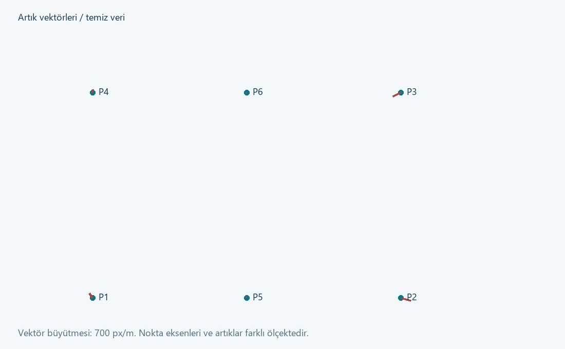
These synthetic datasets were created for this manual; they are neither field coordinates nor official calibration data. Calculations were checked using an independent reference least-squares solution. The live KGT interface was not operated or numerically tested for this study; the following values are references for comparison with the application.
Setup
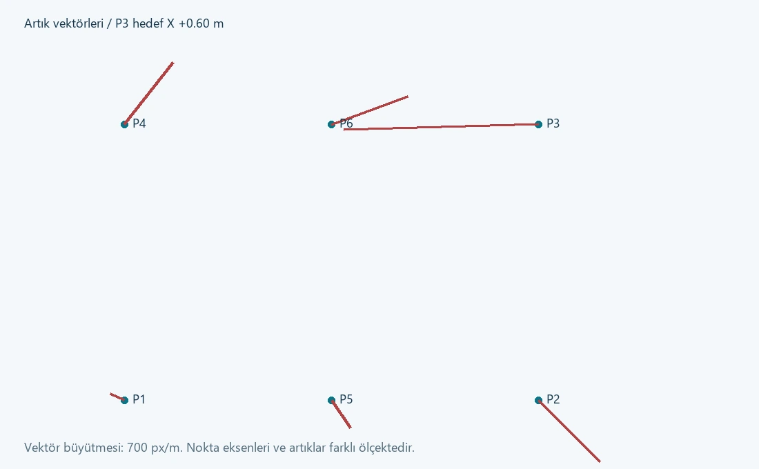
Source points occupy the four corners and midpoints of the lower/upper edges of a 100 × 100 m rectangle. The true model is tx=500 m, ty=1000 m, a=1.0002 and b=0.0003. Synthetic centimetre-level perturbations were added to target coordinates. In the second file, only P3 target X was increased by 0.60 m.
ID   XS      YS       XT(clean)    YT(clean)
P1    0       0       500.010000   999.980000
P2  100       0       600.000000   999.980000
P3  100     100       600.070000  1100.010000
P4    0     100       500.020000  1100.010000
P5   50       0       550.015000   999.980000
P6   50     100       550.035000  1100.010000
The download contains the same six numerical rows. Confirm the reader does not misinterpret the header; if necessary, use only the numeric rows in the working file.
| Quantity | Clean-data reference | Data with +0.60 m added to P3 |
|---|---|---|
| tx [m] | 500.002000 | 499.982000 |
| ty [m] | 999.992000 | 999.992000 |
| a | 1.000260000 | 1.001460000 |
| b | 0.000200000 | 0.001400000 |
| s=√(a²+b²) | 1.000260020 | 1.001460979 |
| θ [degrees] | 0.011456177 | 0.080097097 |
| SSE [m²], P=I | 0.001760 | 0.256160 |
| s₀ [m], f=8 | 0.014832397 | 0.178941331 |
| P3 X residual [m] | −0.022 | −0.402 |
Calculate statistics independently
If prior scalar standard deviation can genuinely be taken as σ₀=0.020 m, this example gives T=0.001760/0.0004=4.4 for clean data and T=640.4 for contaminated data, both with f=8. Compare against the appropriate chi-square limits after defining the hypothesis and α. Using s₀ estimated from the same data again in the denominator does not provide an independent global test; T then equals f by definition.
For P3's X component, Qvv,ii=0.633333333 and contaminated-solution v=−0.402 m give w≈−25.2569. This applies to the known prior scale of 0.020 m. The largest clean-data |w| is approximately 1.7592. This example's σ₀ is not a statement of field accuracy.
KGT comparison protocol
- Load the clean file into the 2D similarity common-point table. Check all six points and their columns.
- Enable the report and solve. Save parameters with sufficient decimals. In this model, scale is s and rotation is expressed in degrees.
- Recalculate all six points from the parameters. For P1, for example: computed (500.002,999.992), observed (500.010,999.980), residual (−0.008,+0.012) m.
- Compare table output and both report residual components against the reference. Do not inspect only the report heading or first residual column.
- Repeat with the contaminated file. Examine parameter changes and effects propagated to other points.
- Omit P3 for investigation only after confirming the known synthetic error. Retain solutions before and after omission.
- At unused points such as Q=(25,25) and Q=(75,75), also compare the estimated model against the true synthetic model. True coordinates are known in this example; field work requires independent measurements.
How to read the computation report
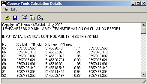
| Report field | Interpretation | Independent check |
|---|---|---|
| Input / identical control points | Common points actually used in the solution | IDs, row count, columns and duplicates |
| Adjusted coordinates | Computed coordinates fitting the chosen model | Recompute from parameters; do not replace original observations |
| Residuals | Differences between modelled and observed coordinates | Verify sign, row and component order by direct subtraction |
| Standard deviations | Precision derived under the relevant stochastic model | Which covariance, scale and degrees of freedom were used? |
| Transformation parameters | Coefficients from the latest successful solution | Units, direction, convention, decimal loss and application test |
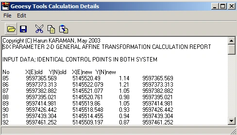
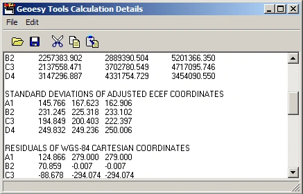
Important implementation limit: reports also need verification
The reviewed 2D reporting paths included cases requiring independent checks of component/row matching for residuals. Therefore, do not use the second residual column alone to accept results or reject points. Calculate XT/YT from the parameters and subtract observed coordinates; compare with table transformation and the report. If inconsistent, do not approve production on the report alone.
RMS and s₀ need not be the same
RMSX = √[Σ ΔXi²/n]           RMSY = √[Σ ΔYi²/n]
RMS2D = √[Σ (ΔXi² + ΔYi²)/n]
s₀ = √[vᵀPv/(m−p)]          [full rank and f>0]
Summarise internal and independent check differences separately. Mean difference indicates bias, RMS overall magnitude and maximum difference the worst point. They describe different things. RMSE alone is not a confidence level without bias and sample size. Contractual point-accuracy criteria must be defined separately.
Minimum handover report contents
- Software version, processing date, operator and immutable identification of all files used.
- Source/target CRS, vertical datum, epoch, axes and units.
- Model, transformation direction, parameter units and rotation convention.
- Included/excluded common points, reasons for exclusion and control geometry.
- Residual table/vectors, statistical assumptions and independent-check results.
- Area of validity, tolerances, final decision and known limitations.
KML, KMZ and DXF: visual overlap is not a survey check
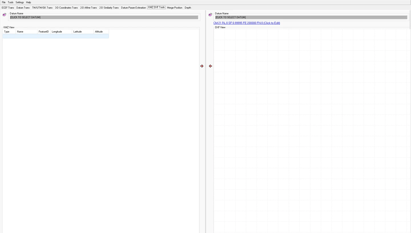
KMZ DXF Toolsprovides table/drawing inspection of KML/KMZ data and prepares exchange with projected CAD data. KML coordinate order is usually longitude, latitude, altitude which may differ from KGT's latitude/longitude input order. DXF coordinates are drawing numbers that cannot be assumed to carry a CRS definition.
 123
- 1 Datum selection for the input side.
- 2 Target datum and TM parameter summary.
- 3 Operation direction.
The empty screen illustrates the controls. Do not start a production transformation while “Click to select datum” indicates an undefined datum.
Development screen archive, 11 February 2026.KMZ → DXF
- Check that the input is at the expected location and verify the meaning of geographic coordinates/heights.
- Select target datum, ellipsoid and TM parameters according to the project definition.
- Check object/point counts in the table and preview. Do not lose unsupported geometry unnoticed.
- Transform/export to a new file with a different name.
- In CAD, verify units, coordinate extent, layers/labels and a known-point distance.
DXF → KMZ
- Verify drawing units (metres/mm/feet), E/N axes and projection definition.
- Define an appropriate local transformation first for engineering coordinates. Changing DXF units is not a datum transformation.
- Select required objects and export supported geometry. Do not assume complex blocks, splines and annotations are retained unchanged.
- Open the KMZ in another viewer and compare point counts, line direction, closed boundaries and several numerical check points.
Altitude and background imagery
KML altitudeMode, clamping to ground and the viewer's terrain model can change displayed elevations. Satellite positional offsets and acquisition dates may also differ. A quay that “fits perfectly” in Google Earth is not evidence of centimetre accuracy; numerical validation at official control points is required.
Georeferencing a BMP map
Image georeferencing relates pixel (u,v) and map (E,N) coordinates. The classical KGT help workflow opens a BMP image, selects Georeferencing from the right-click menu and matches pixel and ground coordinates at three known points, then computes with GeoR . Older help states a restart is needed for changes to take effect; reopen the result to verify behaviour in your version.
E = a0 + a1 u + a2 v
N = b0 + b1 u + b2 v
Image Y usually increases downwards; do not equate pixel direction with north. Three non-collinear matches can determine six parameters exactly, but near-zero internal residuals in that solution do not measure independent accuracy.
- Choose a clear image with adequate resolution and preserve the original.
- Distribute three control points around the image as well as possible. Record pixel-picking uncertainty if a mark's centre is unclear.
- Click a pixel, enter ground E/N in the correct units and add it to the list.
- Check columns and directions for all three matches before running GeoR.
- Reopen the image and test at least one independent point not used in the estimation.
- Inspect distortion at corners and outside the control triangle. Use a more suitable raster method if the required accuracy is not achieved.
Scanning distortion, perspective, paper shrinkage and local defects may not be removed everywhere by one affine model. Do not describe three-point referencing as orthophoto production or photogrammetric rectification. An independent multipoint raster adjustment has not been verified in the interface; do not assume it automatically solves additional points robustly.
SonarMagic: combining position and single-beam depth records
Kordil's official product description states that SonarMagic combines timestamped GNSS GGA and single-beam sounding records, interpolates positions to sounding times and processes depths using water level, transducer draft and sound velocity. Supported sounding record families include SMT, DPT and DBT. Processed data can be exported as CSV for subsequent bathymetric analysis.
Define inputs and sign conventions first
- Time: record date/time system, UTC/local offset, latency and sampling interval.
- Position: GGA latitude/longitude format, N/S–E/W signs, fix quality and gaps.
- Depth: what the instrument reports: depth below transducer, depth with draft/offset applied or another reference.
- Draft: the positive-downward distance from water surface to transducer, consistent with the chosen sign convention.
- Water level: elevation relative to the project vertical datum, not an instrument value relative to an arbitrary zero.
- Sound velocity: the reference velocity used by the instrument and any corrections already applied.
Time interpolation and lost records
t0 ≤ ts ≤ t1
α = (ts − t0)/(t1 − t0)
r(ts) ≈ r(t0) + α [r(t1) − r(t0)]
In the reviewed merge path, sounding time is sought between two position records. Cases exist where no extrapolation is performed and records within large GNSS gaps are skipped. Output counts may therefore be below raw sounding counts. “Processing complete” does not mean every row was accepted. Investigate omitted records by time interval.
HHMMSS and combined date/time notation are not physical seconds. Minute/hour/day boundaries, midnight, repeated times and out-of-order records require independent checks. Do not assume the reviewed workflow corrects every boundary automatically. Verify interpolation with a small known dataset crossing a minute boundary before processing long records.
From depth to bed elevation
zbed = zwater − draft − dcorrected
dcorrected ≈ dlogged × c / cref
This simplified vertical single-beam model takes z positive upwards and draft/depth positive downwards. The reviewed KGT depth path assumes a reference velocity of 1500 m/s. If an instrument uses another reference or supplies already corrected depths, do not apply a correction again without checking. Example: zwater=1.20 m, draft=0.50 m, dlogged=10.00 m and c=1500 m/s give zbed=−9.30 m.
Using an SVP
In the reviewed profile check, depth/sound-velocity rows are interpreted as consecutive integer-metre depths starting at 0 m; velocities are checked within 1300–1600 m/s. This format check does not prove the profile is physically correct, current or representative. Test missing depths, out-of-range observations, malformed rows and profile limits with small datasets.
0 1500.0
1 1499.8
2 1499.6
3 1499.5
This is a format example only, not a field profile. Retain the observation time, location, instrument, depth range and correction history. Do not equate the reviewed depth correction with full ray tracing or a physical propagation model through the complete water column.
Processing protocol
- Preserve raw GNSS and sounding files; preview date/time stamps and message types.
- Choose the correct message filter. Check that a blank or faulty filter does not reject valid rows.
- Document draft, water level and constant sound-velocity/profile selection. Do not apply an instrument offset twice.
- For a short continuous test, manually calculate a known sounding's position and bed elevation.
- Process the long file and inspect input/output counts, GNSS intervals, depth jumps and position continuity.
- Accompany the CSV with explicit metadata defining output CRS and vertical datum.
- Complete bar-check, cross-line, water-level and latency checks under the project's QA procedure.
Corrections outside the assumed scope
Do not assume full heave/roll/pitch corrections, dynamic draft, antenna-to-transducer lever arms, advanced latency estimation or a combined uncertainty budget are automatic in this workflow. GGA mean-sea-level height is not directly ellipsoidal height or elevation in a water-level datum. A field existing in a file does not prove it is used in the intended way.
Batch processing and reproducibility
The preview is not the entire file
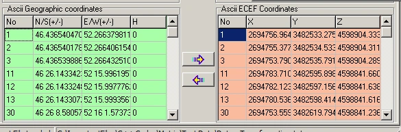
Some large-file reader paths preview only a small section. Do not treat the few visible rows as the total processed count. Check the batch route, output file and row accounting separately. Increase file sizes from verified small tests, considering hardware/memory limits and supported sizes; this manual gives no throughput guarantee.
Create an archive package
Job ID
  raw_data/       unchanged inputs
  definitions/    datum, projection, units, epoch
  checks/         common points and independent checks
  work/           tests and intermediate output
  delivery/       approved results, report, limitations
Retain file hashes, such as SHA-256, and the transformation recipe in a separate job record. Identical filenames do not mean identical contents. Do not store parameters only in screenshots; save numerical values with sufficient precision.
Rounding budget
One arcsecond of latitude is about 31 m; longitude distance depends on latitude. In decimal degrees, 10⁻⁶° can approach a decimetre horizontally. Reprojecting low-precision geographic output causes avoidable losses in precise work. Derive the required decimals from the job accuracy; more displayed digits do not improve physical accuracy.
Minimum transformation test matrix
| Test | Expected check |
|---|---|
| Identity | A point must remain unchanged with identical definitions/systems |
| Pure translation | The same difference at every point |
| Pure scale with zero rotation | Correct length ratio; application and report agree |
| Known rotation / near ±90° | Correct sign, quadrant and inverse direction |
| Blank, malformed or incomplete row | No hidden column shifts or silent data loss |
| Boundary/geometry | Near-collinear control and out-of-coverage points must be recognised |
| Independent real point | Exclude incorrect definitions that nevertheless close in both directions |
Checklists for the processor and reviewer
Checkboxes assist the current session and are not official records. Set acceptance tolerances in advance according to project specifications and risk. This manual does not prescribe one centimetre threshold for every job.
A · Input and definitions
B · Estimation
C · Independent validation
D · Delivery
Do's and don'ts
| Do | Do not |
|---|---|
| Validate with small, known data first. | Do not accept every record merely because a file opens. |
| Read residual patterns together with independent checks. | Do not remove the largest residual without justification. |
| State uncertainty assumptions explicitly. | Do not claim accuracy from decimal counts or small sigmas. |
| Identify corrections already applied by the sonar instrument. | Do not apply draft, sound velocity or height offsets twice. |
| Supply transformation parameters with their area of validity. | Do not extrapolate local agreement to an entire country. |
Trace symptoms back to the root cause
| Symptom | Check sequence | Condition for returning to production |
|---|---|---|
| Empty file / missing rows | Delimiter, decimals, header, filter, supported row format and preview limit | Input, read and output row counts must be reconciled |
| Result far from expected location | E/N or φ/λ, metres/feet/mm, zone, hemisphere and datum direction | Numerical agreement at a known point |
| Inconsistent second residual component in report | Recalculate both components from parameters; verify row/ID matching | No acceptance until report/calculation/application differences are explained |
| Unexpected pure-scale or large-rotation result | Similarity scale/angle display, quadrant and inverse application | All paths must agree in the synthetic reference test |
| No solution / extreme parameters | Point count, collinear/repeated geometry, malformed data and excessive coordinate differences | Adequate rank and physical model; independent checks pass |
| Report warns but parameters are present | Retained prior parameters, initial report text and actual error state | Do not ignore the warning; require a new successful solution and independent check |
| Only height is wrong | h/H, geoid, height units, datum, antenna/draft and unchanged Z carried through 2D | Vertical reference and sign must be verified |
| KMZ appears offset | Projection, units, satellite positional accuracy and local grid | Check numerically; do not fit parameters by imagery alone |
| Sonar output sparse or discontinuous | GNSS gaps, time intervals, malformed messages, filter and ordering | Reasons for omissions and coverage loss documented |
| Position jumps at minute boundaries / midnight | Conversion to physical seconds and interpolation boundary test | Suspend the affected operation until validated with boundary data |
| Slow processing / errors with large files | Small subset, memory, output path and malformed long rows | Never deliver incomplete files; reprocess under controlled conditions |
| Function disabled | Required datum/input, minimum points and About registration status | Use official registration/support; do not bypass licensing checks |
What to include in a support request
Version, Windows details, selected operation, expected/actual result, numeric difference and the smallest anonymised dataset reproducing the issue. Do not send confidential project information, personal data, registration keys or connection credentials. A screenshot alone may be insufficient when parameter direction and units are unclear.
Symbols, sources and version note
| Symbol | Definition |
|---|---|
| φ, λ, h / H / N | Latitude, longitude, ellipsoidal height / orthometric height / geoid undulation |
| a, f, ν | Ellipsoid semi-major axis, flattening and prime-vertical radius of curvature |
| E, N / X,Y,Z | Easting and northing / Cartesian components according to context |
| A, P, l, q, v | Design matrix, weights, observations, parameters and corrections/residuals |
| Q / C | Cofactor / covariance matrix; do not confuse scales |
| n / m / p / f | Number of points / scalar observations / parameters / degrees of freedom |
| σ₀ / s₀ | Prior reference standard deviation / posterior estimate |
| θ, s, dS | Rotation, scale factor and ppm scale difference; units depend on context |
Symbol reuse: N may mean geoid undulation, northing or normal matrix in different sections; a may mean ellipsoid semi-major axis or a similarity coefficient. Use the local definition in each equation. Do not equate height h with statistical leverage.
Sources
- Kordil Geodesy Tools — official product page. Capability summary, official interface image, distribution and support information.
- Existing KGT help, screen archive and sample datasets. Historical help was compared with the current program structure, and old free-distribution/registration instructions were distinguished from the current product page.
- IOGP / EPSG Guidance Note 7-2 — Coordinate Conversions and Transformations Including Formulas. Standard reference for coordinate operations and mathematical conventions.
- PROJ — Helmert Transformation. Technical reference for conventions, units and operation direction; this does not claim KGT uses PROJ.
Distribution and registration
The official product page describes KGT as freely distributed Windows software. For the current installer, documentation and registration assistance, use geodesytools@kordil.com or the official process in the application's About window. Do not substitute old package instructions for current licence terms.
Limits of this publication
This manual was prepared by reviewing the current program structure, forms, mathematical calculation paths, help assets and Kordil product information. No source files were changed, no new adjustment capability was added and no new software release was issued. Source review does not replace live-interface or field acceptance testing.
Web/PDF publication checks and independent mathematical verification of synthetic examples do not certify every algorithm in the KGT executable. In particular, report-component matching, pure scale/large rotations, global ECEF inverse limits and time boundaries must be tested in the application before production use.
Kordil Geodesy Tools is a software product developed by Kordil. Other language editions of this guide are available from the language menu. This publication does not assume registered trademark status for other products.